Creating Distributions Using Machine Learning
This method of creating a distribution is available from Simul8 2022 onwards, allowing you to use machine learning algorithms to create a distribution for use in your simulation.

To create a distribution using Machine Learning algorithms, you can either use R or Python.
If using R, the ML algorithm must be part of a function which is saved as an .RDS file. The function must also be able to read in a dataframe, with the parameter name in column 1 and the parameter value in column 2. For Python, the algorithm must be saved in a .py file and the function must be called prediction. It also must take in two lists as the arguments.
Note: for both, your Machine Learning algorithm must return a number.
Setup
To create a distribution, navigate to the ‘Data and Rules’ tab and select ‘Create Distribution’. Next, give your distribution a name, then select the option ‘Machine Learning’ and click ‘Next’. By default, Simul8 will use R. If you want to use Python, click on Advanced Settings.
In the Setup tab, click on Browse and select the file which contains your algorithm. Then add the simulation parameters the algorithm needs. Click Add, this will open a new dialog. Give you parameter a name and a value – the value will usually be a Label, spreadsheet location or object property.
The name should come from the variable used to train the algorithm. It is important that the spelling used is the same as in R or Python when training the algorithm. As always in Simul8, this distribution can now be selected in many places in your simulation, e.g., for timings, breakdowns, batching out etc..
Tutorial using R
In this tutorial we will show you how you can use Machine Learning to control the timing of a checkout counter in a simulation.
What you will need to complete this tutorial:
R
Step 1: Create your Machine Learning algorithm
We will use a Decision Tree to create a ML algorithm based on the data in the CheckOut_Data file. Open R and copy and paste the script below into your R console, making sure you update the directory to where you saved the CheckOut_Data.xlsx file, then Run the script.
Note: make sure each folder in your directory is separated by two backslashes (\\)
library(readxl)
library(rpart)
library(rpart.plot)
#change this directory to one where you have saved CheckOut_Data.xlsx
directory = “C:\\Users\\yourname\\Downloads”
path = (paste(directory,“\\CheckOut_Data.xlsx”,sep = “”))
DTData = as.data.frame(read_excel(path,sheet = “Sheet1”))
set.seed(1234)
tree = rpart(Time ~., data = DTData)
rpart.plot(tree)
path = (paste(directory,“\\GetTimeDT.rds”,sep = “”))
saveRDS(tree,path)
Step 2: Create a prediction function
Open a new R Script, copy and paste the below script into the console, and update the directories. Now run the script.
Timing = function(df){
Return = (df[1,2])
Items = (df[2,2])
#change this rds file to the same .RDS you have just created
algorithm = readRDS(“C:\\Users\\yourname\\Downloads\\GetTimeDT.rds”)
data = data.frame(Return, Items)
return(predict(algorithm,data))
}
#change this directory to a location on your machine. this is the file you will use for Simul8
saveRDS(Timing,“C:\\Users\\yourname\\Desktop\\GetTimeRF.rds”)
This creates your .RDS file that you will choose in your simulation (see next step).
Step 3: Apply the Machine Learning algorithm in the simulation
Open the Check Out simulation, navigate to the ‘Data and Rules’ tab and select ‘Create Distribution’. Next, give your distribution a name, then select the option ‘Machine Learning’ and click ‘Next’.
Click on Add and enter the parameters. Type the Name (Returns), then click on the Value field and onto the button to its right – this will open the Formula Editor. Choose Labels and double-click on lbl_return, then click OK.
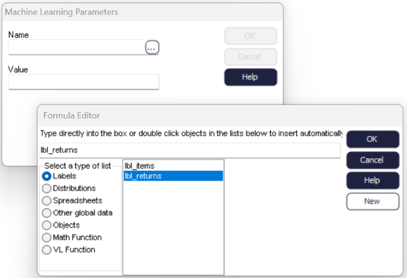
Now do the same for Items. Enter the name as Items, open the Formula Editor from the Value field, choose Labels and double-click on lbl_items. Click OK. Then go to the Check Out Activity, select the distribution on the timing and select the new Machine Learning -based distribution as the timing.
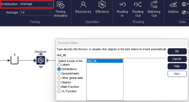
Reset and run your simulation. The timing of the Check Out Activity will now follow the ML algorithm we have created.
Tutorial using Python
In this tutorial we will show you how you can use Machine Learning to control the timing of a checkout counter in a simulation.
What you will need to complete this tutorial:
Python
Step 1: Create your Machine Learning algorithm
Open your preferred Python interface, such as Jupiter notebook or Visual studio, in this example we will use Jupiter. We will use a Decision Tree to create a ML algorithm based on the data in the CheckOut_Data file. Copy and paste the script below into your notebook.
#First, we need to load in the packages needed for a decision tree
import pandas as pd
from sklearn import tree
from sklearn.tree import DecisionTreeClassifier
import pickle
#Then we lock in the file path, when saving this as a py file by using the download section remove the “” as this is only needed in Jupiter notebook
filepath = os.path.dirname(os.path.abspath(“file”))
# Read in the data and save as a name, in this case df for dataframe was used
df = pd.read_csv(filepath+r'\ CheckOut_Data.csv')
features = ['Return','Items']
X = df[features].values
y = df['Time']
# Then make the model based on the x and y data arrays in this case a decision tree
from sklearn.svm import SVC
from sklearn.pipeline import make_pipeline
from sklearn.preprocessing import StandardScaler
dtree=clf = make_pipeline(StandardScaler(), SVC(gamma='auto'))
dtree=clf.fit(X, y)
dtree = DecisionTreeClassifier(max_depth = 2,max_leaf_nodes=10)
dtree = dtree.fit(X,y)
# Save the tree as a sav file which we will use in the prediction function
filename = filepath+r'\TimeDT.sav'
pickle.dump(dtree,open(filename,'wb'))
Step 2: Create a prediction function
Now open a new Script, copy and paste the below script into the console, and run the script. Remember to change (file) to (“file”) if running in a Jupiter notebook. For Simul8 to be able to run it save the scripts as a .py file.
import pickle
import os
def prediction(list1,list2):
filepath = os.path.dirname(os.path.abspath(file))
filename = filepath+r'\TimeDT.sav'
loaded_model = pickle.load(open(filename,'rb'))
result = loaded_model.predict([list2])
return result[0]
When using Python, the script to create the prediction model for timing data is shorter than in R. However, to work correctly it is necessary that Python is installed directly onto the machine together with all necessary packages through the Command Prompt.
Step 3: Apply the Machine Learning algorithm in the simulation
Open the Check Out simulation, navigate to the ‘Data and Rules’ tab and select ‘Create Distribution’. Next, give your distribution a name, then select the option ‘Machine Learning’ and click ‘Next’. Select Advanced and choose Python.
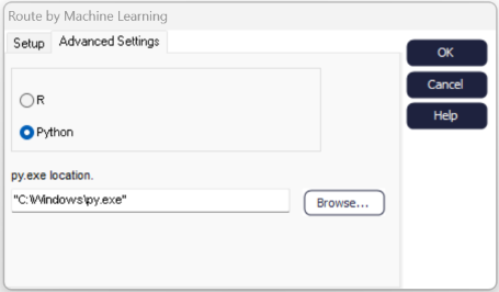
Go back to setup, click on Browse and find the prediction.py script file you saved in step 2. Click on Add and enter the parameters. Type the Name (Returns), then click on the Value field and on the button to its right – this will open the Formula Editor. Choose Labels and double-click on lbl_return, then click OK.

Now do the same for Items. Enter the name as Items, open the Formula Editor from the Value field, choose Labels and double-click on lbl_items. Click OK. Then go to the Check Out Activity, select the distribution on the timing and select the new machine learning based distribution as the timing. Click OK

Reset and run your simulation. The timing of the Check Out Activity will now follow the machine learning algorithm we have created.
Having trouble setting up Distribution By ML? Check out our Machine Learning Troubleshooting page for more help.
Note creating a distribution using ML is not available in Simul8 Online.